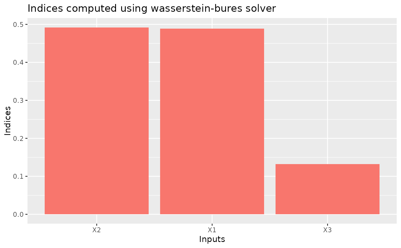
Plot optimal transport sensitivity indices — plot.gsaot

Plot Optimal Transport based sensitivity indices using ggplot2 package.

Usage

# S3 method for class 'gsaot_indices'
plot(x, ranking = NULL, wb_all = FALSE, threshold = NULL, ...)

Arguments

x: An object generated by ot_indices, ot_indices_1d, or ot_indices_wb.
ranking: An integer with absolute value less or equal than the number of inputs. If positive, select the first ranking inputs per importance. If negative, select the last ranking inputs per importance.
wb_all: (default FALSE) Logical that defines whether or not to plot the Advective and Diffusive components of the Wasserstein-Bures indices.
threshold: (default NULL) A double or and object of class gsaot_indices that represents a lower threshold.
...: Further arguments passed to or from other methods.

Value

A ggplot object that, if called, will print

Examples

N <- 1000

mx <- c(1, 1, 1)
Sigmax <- matrix(data = c(1, 0.5, 0.5, 0.5, 1, 0.5, 0.5, 0.5, 1), nrow = 3)

x1 <- rnorm(N)
x2 <- rnorm(N)
x3 <- rnorm(N)

x <- cbind(x1, x2, x3)
x <- mx + x %*% chol(Sigmax)

A <- matrix(data = c(4, -2, 1, 2, 5, -1), nrow = 2, byrow = TRUE)
y <- t(A %*% t(x))

x <- data.frame(x)

M <- 25

# Calculate sensitivity indices
sensitivity_indices <- ot_indices_wb(x, y, M)
sensitivity_indices
#> Method: wass-bures 
#> 
#> Indices:
#>        X1        X2        X3 
#> 0.4784630 0.5223975 0.1221244 
#> 
#> Advective component:
#>        X1        X2        X3 
#> 0.2948087 0.3300739 0.1068931 
#> 
#> Diffusive component:
#>         X1         X2         X3 
#> 0.18365431 0.19232354 0.01523135 

plot(sensitivity_indices)