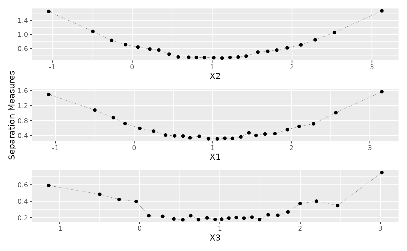
Plot optimal transport local separations — plot

Plot Optimal Transport based local separations for each partition using ggplot2 package. If provided, it plots also the uncertainty estimates.

Usage

plot_separations(x, ranking = NULL, wb_all = FALSE, ...)

Arguments

x: An object generated by ot_indices, ot_indices_1d, or ot_indices_wb.
ranking: An integer with absolute value less or equal than the number of inputs. If positive, select the first ranking inputs per importance. If negative, select the last ranking inputs per importance.
wb_all: (default FALSE) Logical that defines whether or not to plot the Advective and Diffusive components of the Wasserstein-Bures indices.
...: Further arguments passed to or from other methods.

Value

A patchwork object that, if called, will print.

Examples

N <- 1000

mx <- c(1, 1, 1)
Sigmax <- matrix(data = c(1, 0.5, 0.5, 0.5, 1, 0.5, 0.5, 0.5, 1), nrow = 3)

x1 <- rnorm(N)
x2 <- rnorm(N)
x3 <- rnorm(N)

x <- cbind(x1, x2, x3)
x <- mx + x %*% chol(Sigmax)

A <- matrix(data = c(4, -2, 1, 2, 5, -1), nrow = 2, byrow = TRUE)
y <- t(A %*% t(x))

x <- data.frame(x)

M <- 25

# Get sensitivity indices
sensitivity_indices <- ot_indices(x, y, M)
plot_separations(sensitivity_indices)